Machine Learning analysis¶

This is a Python base notebook

Kaggle’s Spotify Song Attributes dataset contains a number of features of songs from 2017 and a binary variable target that represents whether the user liked the song (encoded as 1) or not (encoded as 0). See the documentation of all the features here.

Imports¶

Import libraries¶

import matplotlib.pyplot as plt
import numpy as np
import pandas as pd
from sklearn.compose import ColumnTransformer, make_column_transformer

from sklearn.model_selection import (
    RandomizedSearchCV,
    cross_validate,
    train_test_split,
)
from sklearn.pipeline import make_pipeline 
from sklearn.preprocessing import StandardScaler, OneHotEncoder
from sklearn.impute import SimpleImputer
    
from sklearn.dummy import DummyClassifier
from sklearn.linear_model import LogisticRegression, Ridge
from sklearn.ensemble import RandomForestClassifier
from lightgbm.sklearn import LGBMClassifier
from xgboost import XGBClassifier
from catboost import CatBoostClassifier
from sklearn.tree import DecisionTreeClassifier
from sklearn.ensemble import VotingClassifier

from sklearn.metrics import (
    classification_report,
    roc_curve,
    RocCurveDisplay,
    roc_auc_score
)

import shap
from pylyrics import clean_text as ct

def mean_std_cross_val_scores(model, X_train, y_train, **kwargs):
    """
    Returns mean and std of cross validation

    Parameters
    ----------
    model :
        scikit-learn model
    X_train : numpy array or pandas DataFrame
        X in the training data
    y_train :
        y in the training data

    Returns
    ----------
        pandas Series with mean scores from cross_validation
    """

    scores = cross_validate(model, X_train, y_train, **kwargs)

    mean_scores = pd.DataFrame(scores).mean()
    std_scores = pd.DataFrame(scores).std()
    out_col = []

    for i in range(len(mean_scores)):
        out_col.append((f"%0.3f (+/- %0.3f)" % (mean_scores[i], std_scores[i])))

    return pd.Series(data=out_col, index=mean_scores.index)

Reading the data CSV¶

Read in the data CSV and store it as a pandas dataframe named spotify_df.

spotify_df = pd.read_csv('data/spotify_df_processed.csv')#, index_col = 0 )
spotify_df.head(6)

	acousticness	danceability	duration_ms	energy	instrumentalness	key	liveness	loudness	mode	speechiness	...	emb_sent_758	emb_sent_759	emb_sent_760	emb_sent_761	emb_sent_762	emb_sent_763	emb_sent_764	emb_sent_765	emb_sent_766	emb_sent_767
0	0.0102	0.833	204600	0.434	0.0219	2	0.165	-8.795	1	0.431	...	-0.043803	-0.447969	0.751878	-0.143682	-0.581485	-0.016169	0.619145	0.287845	-0.234614	-0.471101
1	0.0102	0.833	204600	0.434	0.0219	2	0.165	-8.795	1	0.431	...	-0.242343	0.043233	0.199484	0.161576	-0.384538	0.126095	0.462813	0.112398	0.002923	-0.256447
2	0.0102	0.833	204600	0.434	0.0219	2	0.165	-8.795	1	0.431	...	-0.316598	-0.339585	0.321482	0.280396	-0.003586	0.132081	-0.445193	0.301628	-0.287356	-0.504784
3	0.0102	0.833	204600	0.434	0.0219	2	0.165	-8.795	1	0.431	...	0.087176	-0.227342	0.278918	0.479892	-0.431301	0.224406	1.213418	-0.474493	-0.316002	-0.365130
4	0.0102	0.833	204600	0.434	0.0219	2	0.165	-8.795	1	0.431	...	0.117087	-0.418446	-0.040964	0.428880	-0.310667	-0.276378	0.260933	-0.361207	-0.267050	-0.332415
5	0.0102	0.833	204600	0.434	0.0219	2	0.165	-8.795	1	0.431	...	-0.182009	-0.468775	0.299990	0.213028	0.011709	-0.149237	0.507415	0.057419	-0.013157	-0.161389

6 rows × 1646 columns

Data splitting¶

Split the data into train and test portions. Remove song_title, separate data to X_train, y_train, X_test, y_test.

train_df, test_df = train_test_split(spotify_df, test_size=0.2, random_state=123)
X_train, y_train = train_df.drop(columns=["target"]), train_df["target"].astype('category')
X_test, y_test = test_df.drop(columns=["target"]), test_df["target"].astype('category')

# printing the number of observations for train and test sets
print('The number of observations for train set: ', train_df['target'].shape[0])
print('The number of observations for test set: ', test_df['target'].shape[0])

The number of observations for train set:  3831
The number of observations for test set:  958

I split 20% of the observations in the test data and 80% in the train data set. Overall the data set has about 4,000 observations, as it is not a very large data set, I preserved more portion for training.

Scoring metric¶

print('The number of observations for positive targe: ', train_df["target"].sum())
print('The number of observations for negative targe: ', len(train_df["target"])-train_df["target"].sum())

The number of observations for positive targe:  1993
The number of observations for negative targe:  1838

Since it is a balanced data set and both positive and negative class are equally balanced, accuracy and precision-recall curves are selected as scoring metric.

scoring_metric = ["accuracy", "roc_auc"]

Preprocessing and transformations¶

Here is different feature types and the transformations I will apply on each feature type.

Transformation	Reason	Features
OneHotEncoder	All of these features have fixed number of categories. `key` is circulated features like months.	`key`
StandardScaler	Numeric columns needs standardization	`acousticness`, `danceability`, `duration_ms`, `energy`, `instrumentalness`, `liveness`, `loudness`, `mode`, `speechiness`, `tempo`, `time_signature`, `valence`
SimpleImputer, StandardScaler	Analyze lyrics word using `paraphrase-distilroberta-base-v1`, Numeric feature, processed in feature engineering	`emb_sent_`
none	The format are as required, represented as category features, processed in feature engineering	`genres_`
drop	Free text column which has low correlation with target.	`song_title`
drop	Replaced by artist genres `genres_`, do not want to be bounded by specific artist	`artist`

category_feats = ["key"]
none_feats = [col for col in X_train.columns if col.startswith('genres_')]
drop_feats = ['song_title', "artist", 'lyrics'] # Don't want to be bounded by artist


numeric_feats  = list(set(X_train.columns)
            - set(category_feats)
            - set(none_feats)
            - set(drop_feats)
        )

numeric_pipe = make_pipeline(SimpleImputer(missing_values=np.nan, strategy='mean'), StandardScaler())


preprocessor = make_column_transformer(
    ("drop", drop_feats),
    (numeric_pipe, numeric_feats),
    (OneHotEncoder(handle_unknown="ignore", sparse=False), category_feats),
    ("passthrough", none_feats)
)
preprocessor.fit(X_train, y_train);

Baseline model¶

results = {}

dummy = DummyClassifier()
baseline_pipe = make_pipeline(preprocessor, dummy)
results['dummy'] = mean_std_cross_val_scores(make_pipeline(preprocessor, dummy), X_train, y_train, 
                                             return_train_score=True, scoring=scoring_metric)

pd.DataFrame(results)

	dummy
fit_time	0.138 (+/- 0.015)
score_time	0.054 (+/- 0.003)
test_accuracy	0.520 (+/- 0.001)
train_accuracy	0.520 (+/- 0.000)
test_roc_auc	0.500 (+/- 0.000)
train_roc_auc	0.500 (+/- 0.000)

Accuracy of Dummy classifier depends on class ratio. As we have a balanced data set, the accuracy of Dummy classifier is around 50%.

Linear models¶

Model training - LogisticRegression¶

First, a linear model is used as a first real attempt. Hyperparameter tuning is also carried out for tuning to explore different values for the regularization hyperparameter. Cross-validation scores along with standard deviation and results summary is shown in below.

#pipe logistic regression
pipe_logisticregression = make_pipeline(preprocessor,
                           LogisticRegression(max_iter=2000, 
                                             random_state=123))

#save in the results logistic regression score
results["LogisticReg"] = mean_std_cross_val_scores(pipe_logisticregression, 
                                                   X_train, 
                                                   y_train, 
                                                   return_train_score=True,
                                                   scoring = scoring_metric,
                                                   n_jobs=-1)
pd.DataFrame(results)

	dummy	LogisticReg
fit_time	0.138 (+/- 0.015)	13.436 (+/- 0.415)
score_time	0.054 (+/- 0.003)	0.138 (+/- 0.048)
test_accuracy	0.520 (+/- 0.001)	0.887 (+/- 0.006)
train_accuracy	0.520 (+/- 0.000)	0.972 (+/- 0.002)
test_roc_auc	0.500 (+/- 0.000)	0.955 (+/- 0.005)
train_roc_auc	0.500 (+/- 0.000)	0.997 (+/- 0.000)

hyperparameter optimization¶

We will carry out hyperparameter optimization: C controls the regularization, and class_weight hyperparameter for tackling class imbalance.

#parameters for logistic regression
param_dist_lg = {'logisticregression__C': np.linspace(2, 3, 6),
                 'logisticregression__class_weight': ['balanced', None]}

#randomized search to find the best parameters
random_search_lg = RandomizedSearchCV(
    pipe_logisticregression, 
    param_dist_lg,
    n_jobs=-1,
    return_train_score=True,
    scoring = scoring_metric,
    refit='accuracy',
    random_state=123
)

random_search_lg.fit(X_train, y_train)
print("Best parameter values are:", random_search_lg.best_params_)
print("Best cv score is:", random_search_lg.best_score_)

Best parameter values are: {'logisticregression__class_weight': None, 'logisticregression__C': 2.8}
Best cv score is: 0.8885437481490055

results['LogisticReg_opt'] = mean_std_cross_val_scores(random_search_lg, 
                                                       X_train, 
                                                       y_train, 
                                                       return_train_score=True,
                                                       scoring = scoring_metric,
                                                       n_jobs=-1) 

pd.DataFrame(results)

	dummy	LogisticReg	LogisticReg_opt
fit_time	0.138 (+/- 0.015)	13.436 (+/- 0.415)	729.602 (+/- 1.470)
score_time	0.054 (+/- 0.003)	0.138 (+/- 0.048)	0.126 (+/- 0.062)
test_accuracy	0.520 (+/- 0.001)	0.887 (+/- 0.006)	0.888 (+/- 0.008)
train_accuracy	0.520 (+/- 0.000)	0.972 (+/- 0.002)	0.974 (+/- 0.003)
test_roc_auc	0.500 (+/- 0.000)	0.955 (+/- 0.005)	0.954 (+/- 0.005)
train_roc_auc	0.500 (+/- 0.000)	0.997 (+/- 0.000)	0.998 (+/- 0.000)

We can see that with optimized hyperparameters, Logistic Regression is doing a bit better. However, it is obvious that we are dealing with overfitting (big gap between test and training scores and the training accuracy is almost 100%). The std is very small ranging in +- 0.01.

print(
    classification_report(
        y_train,
        random_search_lg.predict_proba(X_train)[:, 1] > 0.5,
        target_names=["0", "1"],
    )
)

              precision    recall  f1-score   support

           0       0.97      0.97      0.97      1838
           1       0.97      0.97      0.97      1993

    accuracy                           0.97      3831
   macro avg       0.97      0.97      0.97      3831
weighted avg       0.97      0.97      0.97      3831

fpr, tpr, _ = roc_curve(
    y_train,
    random_search_lg.predict_proba(X_train)[:, 1],
    pos_label=random_search_lg.classes_[1],
)
print(
    "Area under the curve (AUC): {:.3f}".format(
        roc_auc_score(y_train, random_search_lg.predict_proba(X_train)[:, 1])
    )
)
roc_display = RocCurveDisplay(fpr=fpr, tpr=tpr).plot()

Area under the curve (AUC): 0.997

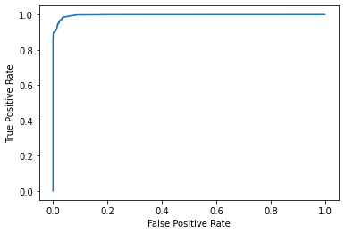
We have high score in AUC and classification report, which means our prediction model performance is good.

Model interpretation on Training set¶

Most important features are listed in below.

col_name_pp_all = [
    *numeric_feats,
    *random_search_lg.best_estimator_.named_steps["columntransformer"]
    .named_transformers_["onehotencoder"]
    .get_feature_names_out(),
    *none_feats
]

data = {
    "Importance": random_search_lg.best_estimator_.named_steps[
        "logisticregression"
    ].coef_[0],
}
feat_importance = pd.DataFrame(data=data, index=col_name_pp_all).sort_values(
    by="Importance", ascending=False
)

feat_importance_200 = pd.concat([feat_importance[0:100], feat_importance[-100:]])
feat_importance_200["rank"] = feat_importance_200["Importance"].rank(ascending=False)
feat_importance_200["side"] = np.where(
    feat_importance_200["Importance"] > 0, "pos", "neg"
)
feat_importance_200

	Importance	rank	side
genres_escape room	1.945204	1.0	pos
genres_chillwave	1.834105	2.0	pos
genres_moombahton	1.747695	3.0	pos
genres_alternative hip hop	1.667970	4.0	pos
genres_motown	1.571681	5.0	pos
...	...	...	...
genres_neo soul	-1.443566	196.0	neg
genres_pop edm	-1.803435	197.0	neg
genres_post-teen pop	-1.932468	198.0	neg
genres_korean pop	-1.965004	199.0	neg
key_0	-2.526168	200.0	neg

200 rows × 3 columns

Most of the important features are determined by genres. Excluding all the features from artist, the other important features are key, danceability and duration. However, the ranking of importance are pretty low, starting from #423.

feat_importance_reset = feat_importance.reset_index()
feat_importance_reset[feat_importance_reset['index'].str.match('^(?![genres])')]

	index	Importance
17	key_4	1.274235
36	loudness	0.948385
41	key_9	0.912684
50	danceability	0.862934
62	key_10	0.789978
114	key_7	0.593926
119	key_5	0.579661
131	instrumentalness	0.537758
132	tempo	0.524994
391	valence	0.198514
582	key_8	0.093041
588	duration_ms	0.089473
612	key_6	0.074142
648	key_11	0.060494
668	liveness	0.047821
1097	mode	-0.057934
1185	key_2	-0.113133
1277	time_signature	-0.173913
1331	acousticness	-0.213958
1611	key_3	-0.780837
1629	key_1	-0.957019
1652	key_0	-2.526168

import altair as alt

base = (
    alt.Chart(feat_importance_200.reset_index())
    .mark_bar()
    .encode(
        x=alt.X(
            "index",
        ),
        y="Importance:Q",
        color="side",
    )
    .properties(height=200, width=800, title="Top 200 important features")
)

brush = alt.selection_interval(encodings=["x"])
lower = (
    base.encode(
        x=alt.X(
            "index",
            axis=alt.Axis(labels=False, title="Features"),
            sort=alt.SortField(field="rank", order="ascending"),
        )
    )
    .properties(height=60, width=800, title="Drag the plot in below to zoom")
    .add_selection(brush)
)

upper = base.encode(
    alt.X(
        "index",
        scale=alt.Scale(domain=brush),
        axis=alt.Axis(title=""),
        sort=alt.SortField(field="rank", order="ascending"),
    )
)

upper & lower

Top 200 most important features are based on genres.

Non-linear models¶

Model training - RandomForestClassifier, XGBClassifier, LGBMClassifier, CatBoostClassifier¶

Second, four non-linear model are trained aside from the linear model above.
After that, feature selection and hyperparameter tuning will carried out in later stage. Cross-validation scores along with standard deviation and results summary is shown in below.

# Random Forest pipe
pipe_rf = make_pipeline(preprocessor, RandomForestClassifier(random_state=123))

# XGBoost pipe
pipe_xgb = make_pipeline(
    preprocessor,
    XGBClassifier(
        random_state=123, eval_metric="logloss", verbosity=0, use_label_encoder=False
    ),
)

# LGBM Classifier pipe
pipe_lgbm = make_pipeline(preprocessor, LGBMClassifier(random_state=123))

# Catboost pipe
pipe_catb = make_pipeline(preprocessor, CatBoostClassifier(verbose=0, random_state=123))

models = {
    "RandomForest": pipe_rf,
    "XGBoost": pipe_xgb,
    "LGBM": pipe_lgbm,
    "Cat_Boost": pipe_catb,
}

# summarize mean cv scores in result_non_linear
for (name, model) in models.items():
    results[name] = mean_std_cross_val_scores(
        model, X_train, y_train, return_train_score=True, scoring=scoring_metric
    )

pd.DataFrame(results)

	dummy	LogisticReg	LogisticReg_opt	RandomForest	XGBoost	LGBM	Cat_Boost
fit_time	0.138 (+/- 0.015)	13.436 (+/- 0.415)	729.602 (+/- 1.470)	3.025 (+/- 0.158)	6.629 (+/- 0.337)	2.496 (+/- 0.136)	43.591 (+/- 0.065)
score_time	0.054 (+/- 0.003)	0.138 (+/- 0.048)	0.126 (+/- 0.062)	0.096 (+/- 0.003)	0.072 (+/- 0.003)	0.061 (+/- 0.003)	0.675 (+/- 0.045)
test_accuracy	0.520 (+/- 0.001)	0.887 (+/- 0.006)	0.888 (+/- 0.008)	0.900 (+/- 0.011)	0.944 (+/- 0.007)	0.950 (+/- 0.003)	0.954 (+/- 0.005)
train_accuracy	0.520 (+/- 0.000)	0.972 (+/- 0.002)	0.974 (+/- 0.003)	0.997 (+/- 0.001)	0.997 (+/- 0.001)	0.997 (+/- 0.001)	0.995 (+/- 0.001)
test_roc_auc	0.500 (+/- 0.000)	0.955 (+/- 0.005)	0.954 (+/- 0.005)	0.960 (+/- 0.002)	0.986 (+/- 0.001)	0.991 (+/- 0.002)	0.991 (+/- 0.002)
train_roc_auc	0.500 (+/- 0.000)	0.997 (+/- 0.000)	0.998 (+/- 0.000)	1.000 (+/- 0.000)	1.000 (+/- 0.000)	1.000 (+/- 0.000)	1.000 (+/- 0.000)

All the non-linear models are overfitting as all the training scores are close to 1. Compared to most of the models, LGBM and Cat_Boost are two of the most balanced model in performance, it has the highest accuracy and comparatively less overfitting (the gap between train and validation scores is smaller).

Stability of scores is more or less stable, with standard deviation ranging in around 0.06.

The fit time of LGBM is much shorter than Cat_Boost, which is important for the model application, therefore, LGBM is by far the most suitable model.

Model interpretation on Training set¶

Since feature_importance_ is not supported on the models, shap is used to examine the most important features of our best non-linear models.

pipe_lgbm.fit(X_train, y_train);

X_train_enc = pd.DataFrame(
    data=preprocessor.transform(X_train),
    columns=col_name_pp_all,
    index=X_train.index,
)

lgbm_explainer = shap.TreeExplainer(pipe_lgbm.named_steps["lgbmclassifier"])
train_lgbm_shap_values = lgbm_explainer.shap_values(X_train_enc)
shap.summary_plot(train_lgbm_shap_values, X_train_enc, plot_type="bar")

LightGBM binary classifier with TreeExplainer shap values output has changed to a list of ndarray

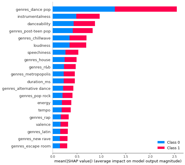
We examined the most important features of LGBMClassifier with SHAP methods. Apart from genre, the results suggests that the most important features are instrumentalness, danceability and loudness. Comparing to the linear model, which suggested all genre_ is the most important features. non-linear model has more diversity.

Model Averaging¶

All the models are overfitted. To ease the fundamental trade off, Averaging is attempted to see if a higher validation score and shorter fit time can be achieved.

avg_classifiers = {
    "random forest": pipe_rf,
    "XGBoost": pipe_xgb,
    "LightGBM": pipe_lgbm
}

averaging_model = VotingClassifier(
    list(avg_classifiers.items()), voting="soft"
) 

results['averaging'] = mean_std_cross_val_scores(
        averaging_model, X_train, y_train, return_train_score=True, scoring=scoring_metric#, cv=2
    )

pd.DataFrame(results)

	dummy	LogisticReg	LogisticReg_opt	RandomForest	XGBoost	LGBM	Cat_Boost	averaging
fit_time	0.138 (+/- 0.015)	13.436 (+/- 0.415)	729.602 (+/- 1.470)	3.025 (+/- 0.158)	6.629 (+/- 0.337)	2.496 (+/- 0.136)	43.591 (+/- 0.065)	14.263 (+/- 0.906)
score_time	0.054 (+/- 0.003)	0.138 (+/- 0.048)	0.126 (+/- 0.062)	0.096 (+/- 0.003)	0.072 (+/- 0.003)	0.061 (+/- 0.003)	0.675 (+/- 0.045)	0.278 (+/- 0.010)
test_accuracy	0.520 (+/- 0.001)	0.887 (+/- 0.006)	0.888 (+/- 0.008)	0.900 (+/- 0.011)	0.944 (+/- 0.007)	0.950 (+/- 0.003)	0.954 (+/- 0.005)	0.951 (+/- 0.004)
train_accuracy	0.520 (+/- 0.000)	0.972 (+/- 0.002)	0.974 (+/- 0.003)	0.997 (+/- 0.001)	0.997 (+/- 0.001)	0.997 (+/- 0.001)	0.995 (+/- 0.001)	0.997 (+/- 0.001)
test_roc_auc	0.500 (+/- 0.000)	0.955 (+/- 0.005)	0.954 (+/- 0.005)	0.960 (+/- 0.002)	0.986 (+/- 0.001)	0.991 (+/- 0.002)	0.991 (+/- 0.002)	0.986 (+/- 0.001)
train_roc_auc	0.500 (+/- 0.000)	0.997 (+/- 0.000)	0.998 (+/- 0.000)	1.000 (+/- 0.000)	1.000 (+/- 0.000)	1.000 (+/- 0.000)	1.000 (+/- 0.000)	1.000 (+/- 0.000)

According to the result, averaging the models neither help the overfitting issue nor scoring. However, the fit time is slower than LGBMClassifier. LGBMClassifier is still the best model.

Results on the test set¶

The best performing model LGBMClassifier is used on the test data and report test scores. Summary is shown as below. Furthermore, some test predictions and corresponding explanation with SHAP force plots are drawn for further study.

#predictions = pipe_catb.predict(X_test)
print("Test Set accuracy: ", round(pipe_lgbm.score(X_test, y_test), 3))

Test Set accuracy:  0.954

The test set score was similar to the validation score. Therefore, the prediction is promising.

Interpretation and feature importances on Test set¶

# Encoding X_test for SHAP force plot
X_test_enc = pd.DataFrame(
    data=preprocessor.transform(X_test),
    columns=col_name_pp_all,
    index=X_test.index,
)
X_test_enc.shape

(958, 1653)

# Create an explainer for X_test_enc
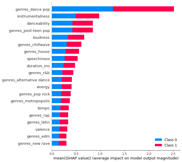
test_lgbm_shap_values = lgbm_explainer.shap_values(X_test_enc)
shap.summary_plot(test_lgbm_shap_values, X_test_enc, plot_type="bar")

LightGBM binary classifier with TreeExplainer shap values output has changed to a list of ndarray

y_test.iloc[8]

# Force Plot for prediction of 4th row (no_default)
shap.force_plot(
    lgbm_explainer.expected_value[1],
    test_lgbm_shap_values[1][8,:],
    X_test_enc.iloc[8,:],
    matplotlib=True,
)

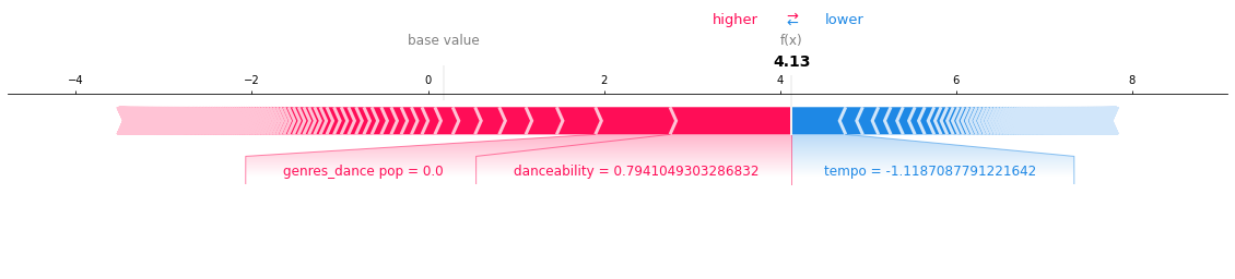
As seen from the plot, the raw score is much smaller than the base value, which predict accurately as Like (class of ‘1’).
danceability and genres_dance_pop are pushing the prediction towards a higher score, and tempo is pushing the prediction towards a lower score.

y_test.iloc[10]

# Force Plot for prediction of 2nd row (no_default)
shap.force_plot(
    lgbm_explainer.expected_value[1],
    test_lgbm_shap_values[1][4,:],
    X_test_enc.iloc[4,:],
    matplotlib=True,
)

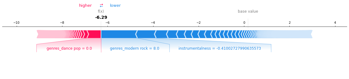
As seen from the plot, the raw score is much smaller than the base value, which predict accurately as Unlike (class of ‘0’).
genres_dance_pop is pushing the prediction towards a higher score, and genres_modern rock and instrumentalness are pushing the prediction towards a lower score.

Summary of machine learning results¶

pd.DataFrame(results)

	dummy	LogisticReg	LogisticReg_opt	RandomForest	XGBoost	LGBM	Cat_Boost	averaging
fit_time	0.138 (+/- 0.015)	13.436 (+/- 0.415)	729.602 (+/- 1.470)	3.025 (+/- 0.158)	6.629 (+/- 0.337)	2.496 (+/- 0.136)	43.591 (+/- 0.065)	14.263 (+/- 0.906)
score_time	0.054 (+/- 0.003)	0.138 (+/- 0.048)	0.126 (+/- 0.062)	0.096 (+/- 0.003)	0.072 (+/- 0.003)	0.061 (+/- 0.003)	0.675 (+/- 0.045)	0.278 (+/- 0.010)
test_accuracy	0.520 (+/- 0.001)	0.887 (+/- 0.006)	0.888 (+/- 0.008)	0.900 (+/- 0.011)	0.944 (+/- 0.007)	0.950 (+/- 0.003)	0.954 (+/- 0.005)	0.951 (+/- 0.004)
train_accuracy	0.520 (+/- 0.000)	0.972 (+/- 0.002)	0.974 (+/- 0.003)	0.997 (+/- 0.001)	0.997 (+/- 0.001)	0.997 (+/- 0.001)	0.995 (+/- 0.001)	0.997 (+/- 0.001)
test_roc_auc	0.500 (+/- 0.000)	0.955 (+/- 0.005)	0.954 (+/- 0.005)	0.960 (+/- 0.002)	0.986 (+/- 0.001)	0.991 (+/- 0.002)	0.991 (+/- 0.002)	0.986 (+/- 0.001)
train_roc_auc	0.500 (+/- 0.000)	0.997 (+/- 0.000)	0.998 (+/- 0.000)	1.000 (+/- 0.000)	1.000 (+/- 0.000)	1.000 (+/- 0.000)	1.000 (+/- 0.000)	1.000 (+/- 0.000)

pd.DataFrame(results).to_csv('data/model_results.csv',index=False)

Spotify User Behaviour Predictor

Machine Learning analysis¶

Imports¶

Import libraries¶

Reading the data CSV¶

Data splitting¶

Scoring metric¶

Preprocessing and transformations¶

Baseline model¶

Linear models¶

Model training - LogisticRegression¶

hyperparameter optimization¶

Model interpretation on Training set¶

Non-linear models¶

Model training - RandomForestClassifier, XGBClassifier, LGBMClassifier, CatBoostClassifier¶

Model interpretation on Training set¶

Model Averaging¶

Results on the test set¶

Interpretation and feature importances on Test set¶

Summary of machine learning results¶